

ML Model Monitoring and Data Drift: PSI, KS Test and Alerts
Monitor ML models in production: data drift vs concept drift, PSI and KS statistics computed by hand in Python, delayed labels, Evidently and Prometheus alerts.
A pressure cooker on a gas stove has a whistle. You do not stand and stare at it for 20 minutes. You go about your work and the whistle tells you when something needs attention. If it never whistles, you check whether the vent is blocked.
Monitoring is the whistle for a deployed model. Nobody can watch thousands of predictions an hour. You decide in advance what "something is wrong" looks like, measure it automatically and get alerted.
What is ML model monitoring?
In the analogy, the whistle is an alert, the pressure is a metric such as drift or error, the number of whistles you wait for is the threshold, and the blocked vent check is monitoring the monitor itself.
ML model monitoring is the continuous measurement of a deployed model's inputs, outputs, performance and serving health, compared with a reference period, so that degradation is detected and acted on before it harms users.
In the first lesson, Chappan Express's eta-model lost accuracy in the monsoon without a single error message. The Kubernetes lesson keeps the pods alive, but a healthy pod can still serve bad predictions. Monitoring is how you see that.
What should you monitor in a production model?
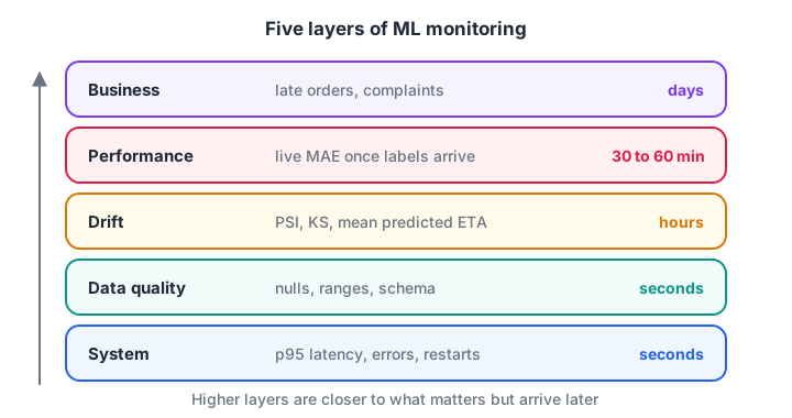
Lower layers are fast and cheap to measure; higher layers are slower but closer to what matters.
| Layer | Example metric for eta-model | Available after | Typical tool |
|---|---|---|---|
| System | p95 latency, error rate, pod restarts | Seconds | Prometheus and Grafana |
| Data quality | Share of null prep_min, distance over 30 km |
Seconds | Validation checks, Evidently |
| Drift | PSI of distance_km, KS of prep_min, mean prediction |
Hours | Evidently, custom jobs |
| Performance | MAE against real delivery minutes | 30 to 60 minutes | Batch job joining predictions to outcomes |
| Business | Share of orders more than 10 minutes late, complaints | Days | Product analytics |
To monitor performance at all, the service must log every prediction with an order ID and model version, and the delivery app must log the real delivery time. A nightly job joins the two.
Data drift vs concept drift
There are several kinds of change, and they need different responses.
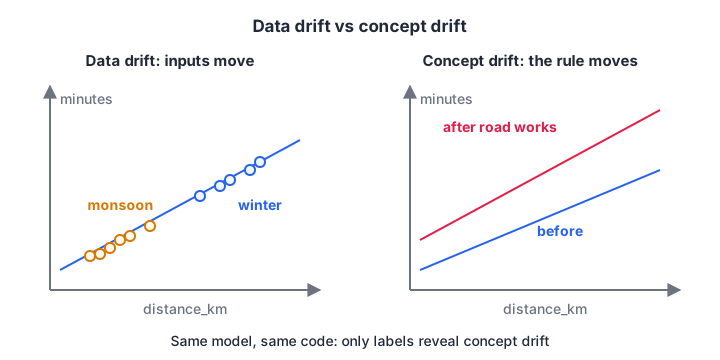
Data drift moves the inputs. Concept drift moves the rule that links inputs to the answer.
| Type | What changes | Chappan Express example | Visible without labels? |
|---|---|---|---|
| Data (covariate) drift | Input distribution P(X) | Monsoon: more short, nearby orders | Yes |
| Prediction drift | Output distribution | Mean predicted ETA rises from 24 to 29 min | Yes |
| Concept drift | Relationship P(y given X) | Road works make rain add 11 min instead of 4 | No, needs labels |
| Label shift | Target distribution P(y) | Festival week: far more long deliveries | Only once labels arrive |
How do you measure data drift?
How to calculate PSI by hand
The Population Stability Index compares two distributions using bins. Split the reference data into bins (often 10 quantile bins), compute the share of reference and current data in each bin, and sum:
PSI = Σ (current% − reference%) × ln(current% / reference%)
A widely used rule of thumb, inherited from credit-scoring practice, reads PSI below 0.1 as stable, 0.1 to 0.25 as a moderate shift and above 0.25 as a major shift. Treat these as starting points and tune them on your own history.
import numpy as np

rng = np.random.default_rng(10)
reference = rng.gamma(shape=3.0, scale=1.3, size=5000)    # distance_km at training
same_week = rng.gamma(shape=3.0, scale=1.3, size=2000)    # a normal week
monsoon = rng.gamma(shape=2.0, scale=1.3, size=2000)      # more short orders

def psi(ref, cur, bins=10, eps=1e-4):
    edges = np.quantile(ref, np.linspace(0, 1, bins + 1))
    edges[0], edges[-1] = -np.inf, np.inf                 # catch out-of-range values
    ref_pct = np.histogram(ref, edges)[0] / len(ref) + eps
    cur_pct = np.histogram(cur, edges)[0] / len(cur) + eps
    return float(np.sum((cur_pct - ref_pct) * np.log(cur_pct / ref_pct)))

def verdict(v):
    return "stable" if v < 0.1 else ("moderate shift" if v < 0.25 else "major shift")

for name, cur in [("normal week", same_week), ("monsoon week", monsoon)]:
    v = psi(reference, cur)
    print(f"{name:13s} PSI = {v:.3f}  -> {verdict(v)}")
The normal week scores close to zero. The monsoon week, with many more short orders, scores far above 0.25. The tiny eps stops a division by zero when a bin is empty, and the open-ended outer bins catch values outside the reference range.
The Kolmogorov-Smirnov test for drift
The KS statistic is the largest vertical gap between the cumulative distribution curves of two samples. It needs no bins, which makes it popular for continuous features. Here it is by hand, checked against scipy.stats.ks_2samp.
import numpy as np
from scipy.stats import ks_2samp

rng = np.random.default_rng(12)
reference = rng.normal(15, 4, 3000)          # prep_min last month
current = rng.normal(16.5, 4, 3000)          # a new restaurant chain joined

def ks_statistic(a, b):
    grid = np.sort(np.concatenate([a, b]))
    cdf_a = np.searchsorted(np.sort(a), grid, side="right") / len(a)
    cdf_b = np.searchsorted(np.sort(b), grid, side="right") / len(b)
    return float(np.max(np.abs(cdf_a - cdf_b)))

print(f"KS by hand : D = {ks_statistic(reference, current):.4f}")
res = ks_2samp(reference, current)
print(f"scipy      : D = {res.statistic:.4f}, p-value = {res.pvalue:.2e}")

for n in (500, 5000, 50000):                 # same 0.2-minute shift, more data
    a, b = rng.normal(15, 4, n), rng.normal(15, 4, n) + 0.2
    r = ks_2samp(a, b)
    print(f"n={n:>6}: D = {r.statistic:.3f}, p-value = {r.pvalue:.4f}")
The hand-written D matches SciPy exactly. The second part shows a trap: the same small 0.2-minute shift goes from "not significant" to "hugely significant" just because there is more data.
With thousands of live predictions a day, almost any feature will show a "significant" p-value. Alert on the size of the shift (D or PSI) with a threshold that matters to the business, not on the p-value alone. The ideas behind p-values are in hypothesis testing.
Quick check
A feature's PSI between training data and last week is 0.31. Using the common rule of thumb, how do you read it?
PSI above 0.25 is conventionally treated as a major shift. Check data quality and performance next.
Concept drift: when inputs look fine but accuracy falls
Drift metrics only watch inputs. In the next block, road works begin on day 8 and rain now delays orders by 11 minutes instead of 4. Distances look the same as always. Only the error, computed once real delivery times arrive, reveals the problem.
import numpy as np
import pandas as pd
from sklearn.linear_model import LinearRegression

rng = np.random.default_rng(14)
def week(n, rain_penalty):
    d = rng.uniform(0.5, 9, n); rain = rng.integers(0, 2, n)
    y = 8 + 3.2 * d + rain_penalty * rain + rng.normal(0, 2.5, n)
    return np.column_stack([d, rain]), y

X0, y0 = week(3000, rain_penalty=4)                   # training period
model = LinearRegression().fit(X0, y0)

rows = []
for day in range(1, 15):
    penalty = 4 if day <= 7 else 11                   # road works from day 8
    X, y = week(400, penalty)                         # same inputs, new relationship
    rows.append({"day": day, "mean_distance": X[:, 0].mean(),
                 "mae": np.abs(y - model.predict(X)).mean()})
daily = pd.DataFrame(rows)
daily["mae_3day"] = daily.mae.rolling(3).mean()
daily["alert"] = daily.mae_3day > 4.0                 # agreed SLO for eta-model
print(daily.round(2).to_string(index=False))
Mean distance barely moves, so PSI would stay quiet. MAE doubles from day 8, and the three-day rolling average crosses the 4-minute target on day 10. The rolling window avoids paging someone over one bad day, at the cost of two days' delay.
This is why performance monitoring with real labels is the final judge. Drift is the early warning; error is the verdict.
Quick check
Input distributions are unchanged but the model's MAE has doubled. What is most likely happening?
The inputs look the same, so the relationship between inputs and outcome must have changed. Only labelled performance metrics reveal this.
Monitoring tools: Evidently and Prometheus
You will not hand-write every metric in production. Two open-source tools cover most needs.
Evidently is a Python library that compares a reference and a current dataset and produces drift and quality reports. With its current API (0.7 and later), a drift report looks like this:
from evidently import Dataset, DataDefinition, Report
from evidently.presets import DataDriftPreset

schema = DataDefinition(numerical_columns=["distance_km", "prep_min", "rider_load"],
                        categorical_columns=["is_raining", "zone"])
reference = Dataset.from_pandas(train_sample_df, data_definition=schema)
current = Dataset.from_pandas(last_week_df, data_definition=schema)

report = Report([DataDriftPreset()])
result = report.run(current, reference)      # current first, then reference
result.save_html("eta_drift_week45.html")
summary = result.dict()                      # feed into alerts or a dashboard
Prometheus collects time-series metrics from your service, and Grafana draws dashboards from them. The official prometheus_client library exposes counters and histograms from the FastAPI app:
from prometheus_client import Counter, Histogram, make_asgi_app

PREDICTIONS = Counter("eta_predictions_total", "Predictions served", ["model_version"])
LATENCY = Histogram("eta_predict_seconds", "Time spent in model.predict")
ETA = Histogram("eta_predicted_minutes", "Predicted delivery minutes",
                buckets=[10, 15, 20, 25, 30, 40, 50, 60, 90])

app.mount("/metrics", make_asgi_app())       # Prometheus scrapes this endpoint

@app.post("/predict")
def predict(order: Order):
    with LATENCY.time():
        eta = float(MODEL["eta"].predict(to_row(order))[0])
    PREDICTIONS.labels(model_version=MODEL["version"]).inc()
    ETA.observe(eta)                         # prediction drift, live
    return {"eta_minutes": round(eta, 1), "model_version": MODEL["version"]}
A Prometheus alerting rule then turns a metric into a page:
groups:
  - name: eta-model
    rules:
      - alert: EtaLatencyP95High
        expr: histogram_quantile(0.95, sum(rate(eta_predict_seconds_bucket[5m])) by (le)) > 0.1
        for: 10m
        labels:
          severity: page
        annotations:
          summary: "eta-model p95 latency above 100 ms for 10 minutes"
For LLM applications, monitoring adds traces, token costs and output quality, covered later in LLM observability.
What to do when a drift alert fires
- Check data quality first. Many "drifts" are broken pipelines: a unit change, a null-filled column, a new app version.
- Check performance. If labels show MAE is still within target, note the drift and keep watching.
- Find the segment. Is it one zone, one restaurant chain, rainy hours only?
- Decide the response. Retrain on recent data, roll back to the previous version, or add a feature (such as a road-works flag).
- Gate the fix. A retrained model goes through the same evaluation gate, automated in CI/CD for machine learning.
Common mistakes in ML monitoring
- Only monitoring uptime. A model can be up and wrong.
- Alerting on p-values. With large samples everything is significant.
- No reference window. Drift needs a baseline, usually the training data or a recent stable month.
- Not logging predictions with IDs. Without them you can never compute real accuracy.
- Too many alerts. People start ignoring them. Alert on a few metrics tied to action.
- Ignoring seasonality. Diwali week always looks different; compare with last year's Diwali, not last week.
To revise the statistics behind these checks, drill statistics-style questions on Debugshala Test. If you want to build a monitoring project with guidance, see hands-on AI training at Debugshala's Old Palasia centre.
Key takeaways
- Monitor five layers: system, data quality, drift, performance and business outcomes.
- Data drift changes inputs; concept drift changes the input-to-target relationship and needs labels to see.
- PSI and the KS statistic are simple to compute and widely used; alert on effect size, not p-values.
- Log predictions with IDs and model versions so they can be joined to real outcomes.
- Every alert should lead to a decision: investigate, retrain, roll back or add features.
FAQ
What is data drift in machine learning?
Data drift is a change in the statistical distribution of a model's input features between training and production. For example, a delivery model trained on winter orders sees far more short rainy-season orders. Drift does not always reduce accuracy, but it is an early warning that the model may be operating outside what it learned.
What is the difference between data drift and concept drift?
Data drift means the inputs change while the input-to-output relationship stays the same. Concept drift means that relationship changes, so the same inputs now lead to different outcomes. Data drift is visible immediately from inputs; concept drift usually shows only when true labels arrive and accuracy drops.
What is a good PSI threshold?
A common rule of thumb treats PSI under 0.1 as stable, 0.1 to 0.25 as a moderate shift and above 0.25 as a major shift. These numbers come from credit-risk practice, so tune them using your own historical data and how sensitive your model is to each feature.
How do you monitor a model when labels arrive late?
Watch what is available immediately: data quality, input drift and prediction drift. Log every prediction with an ID, then join labels when they arrive and compute performance on a rolling window. For very slow labels, use proxy metrics such as complaints or human review of a sample.
Where can I learn ML monitoring and MLOps in Indore?
Debugshala, an IT training and placement institute at Old Palasia in Indore, runs Machine Learning and Generative AI courses in English and Hindi, offline at its campus. Fresh graduates, non-IT learners and people with a year gap are accepted, and a free demo class is offered before enrolment.
From the team behind this site
Go further with the Generative AI Course at Debugshala
These tutorials are written by Debugshala, a training and placement institute at Old Palasia, Indore. The classroom course adds live mentoring, real projects and interview preparation.
- Offline classes at Old Palasia, Indore
- Free demo class before you pay
- Non-IT, fresher and year-gap friendly
- Placement assistance
700+ students placed · 200+ hiring partners · 4.9★ Google rating
