

ML Lifecycle: The 8 Stages of a Machine Learning System
The machine learning lifecycle in 8 stages, from metric and baseline to monitoring and retraining, with runnable Python showing why time-based splits matter.
Think of a new bus route in Indore. Someone decides it should cut travel time from Vijay Nagar to Rajwada by ten minutes. Planners study traffic, draw the route, test it with one bus, launch it, watch the timings for weeks, and redraw it when a flyover opens.
Nobody calls the route "finished" on launch day. Launch is the halfway point.
A machine learning system works the same way. The model you deploy is one pass through a loop that keeps running for as long as the product exists.
What is the ML lifecycle?
In the bus analogy, the ten-minute goal is your success metric, the traffic study is data collection, the trial bus is offline evaluation, launch is deployment, and watching timings is monitoring.
The ML lifecycle is the end-to-end, repeating process of defining, building, deploying, monitoring and improving a machine learning model, where the output of monitoring feeds back into the next round of data and training.
You may have met the data science lifecycle, which ends at insight or a first model. The ML system lifecycle carries on into production. It is the backbone of the MLOps practice introduced in What is MLOps?.
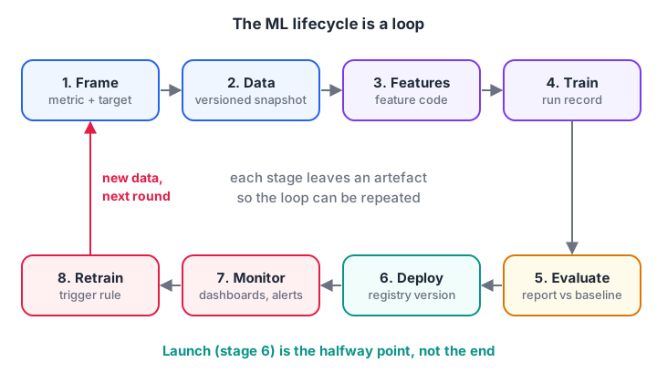
Eight stages, each leaving an artefact. The arrow from monitoring back to data is what makes it a lifecycle.
The 8 stages of the machine learning lifecycle
Here is each stage applied to Chappan Express, the fictional Indore delivery company whose eta-model predicts delivery minutes.
- Frame the problem. Decide what to predict, for whom, and how success is measured. Chappan Express predicts minutes from order to doorstep. Success means a mean absolute error (MAE) under 4 minutes and at least 80% of orders within plus or minus 5 minutes.
- Collect and label data. Gather past orders with their real delivery times. The label is the actual minutes, logged when the rider taps "delivered".
- Prepare data and build features. Clean bad GPS rows, compute distance, add hour of day, rain and rider load.
- Train and experiment. Try a few algorithms and settings. Record every run.
- Evaluate offline. Score on held-out data that imitates the future, against a baseline and the current live model.
- Deploy. Ship the model behind an API, often to a small share of traffic first.
- Monitor. Watch input data, predictions, real delivery times and system health.
- Retrain or retire. When performance drops or new data piles up, start again from stage 2. If the product changes, retire the model.
| Stage | Main question | Artefact left behind |
|---|---|---|
| Frame | What counts as good? | Metric definition and target value |
| Data | What did we learn from? | Versioned data snapshot |
| Features | How were inputs computed? | Feature code and definitions |
| Train | What settings were used? | Run record with params and metrics |
| Evaluate | Is it better than what we have? | Evaluation report |
| Deploy | Which version is live? | Model version in a registry |
| Monitor | Is it still working? | Dashboards and alerts |
| Retrain | When do we refresh? | Trigger rule and new run |
Stage 1 in practice: metrics and a baseline
The most expensive lifecycle mistake is skipping the baseline. If a one-line rule already gets an error of 5 minutes, a model at 4.8 is not worth the servers it runs on.
A good baseline for delivery time is "the median time of past orders at this distance band". The block compares that baseline with a trained model on two metrics: MAE, which engineers like, and the share of orders within 5 minutes, which the business understands.
import numpy as np
import pandas as pd
from sklearn.ensemble import GradientBoostingRegressor
from sklearn.metrics import mean_absolute_error

rng = np.random.default_rng(3)
n = 3000
df = pd.DataFrame({"distance_km": rng.uniform(0.5, 9, n),
                   "prep_min": rng.integers(8, 25, n),
                   "rain": (rng.random(n) < 0.3).astype(int)})
df["minutes"] = (6 + 3.2 * df.distance_km + df.prep_min
                 + df.rain * 5 + rng.normal(0, 3, n))
train, test = df.iloc[:2400], df.iloc[2400:]

# Baseline: median minutes for each 1 km distance band
band = lambda d: d.distance_km.astype(int)
medians = train.groupby(band(train)).minutes.median()
base_pred = band(test).map(medians)

X_cols = ["distance_km", "prep_min", "rain"]
gbr = GradientBoostingRegressor(random_state=0).fit(train[X_cols], train.minutes)
model_pred = gbr.predict(test[X_cols])

for name, pred in [("baseline", base_pred), ("model", model_pred)]:
    mae = mean_absolute_error(test.minutes, pred)
    within5 = (abs(test.minutes - pred) <= 5).mean()
    print(f"{name:9s} MAE {mae:5.2f} min | within 5 min: {within5:.0%}")
The baseline already lands a little above 5 minutes because distance explains a lot. The model roughly halves the error by also using kitchen time and rain. Now the team has a number that justifies the extra work.
Write the metric, the target and the baseline score down before training anything else. Later stages, including the CI gate in the CI/CD lesson, compare against them. For a refresher on MAE and friends, see model evaluation metrics.
Stage 5: why the evaluation split must imitate the future
A model is always used on data from after it was trained. If your test set is a random sample from the same months as training, you are grading it on the past, and the score is too kind.
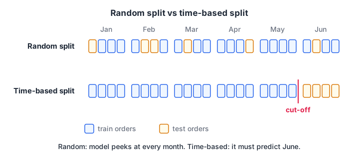
A random split lets the model peek at every month. A time-based split asks the honest question: how well does it do on next month?
Delivery times at Chappan Express creep up as the city grows and new restaurants join far from the centre. The block trains the same model twice, once with a random split and once with a time-based split, and compares the scores.
import numpy as np
import pandas as pd
from sklearn.ensemble import RandomForestRegressor
from sklearn.metrics import mean_absolute_error
from sklearn.model_selection import train_test_split

rng = np.random.default_rng(5)
n = 3000
day = np.sort(rng.integers(0, 180, n))            # 6 months of orders
df = pd.DataFrame({"day": day,
                   "distance_km": rng.uniform(0.5, 9, n),
                   "prep_min": rng.integers(8, 25, n)})
traffic = 0.10 * day                               # city gets busier
df["minutes"] = 6 + 3.2 * df.distance_km + df.prep_min + traffic + rng.normal(0, 3, n)
X, y = df[["day", "distance_km", "prep_min"]], df.minutes

def score(X_tr, X_te, y_tr, y_te):
    m = RandomForestRegressor(n_estimators=40, random_state=0).fit(X_tr, y_tr)
    return mean_absolute_error(y_te, m.predict(X_te))

rand = score(*train_test_split(X, y, test_size=0.2, random_state=0))
cut = df.day < 150                                 # train on first 150 days
time = score(X[cut], X[~cut], y[cut], y[~cut])
print(f"Random split MAE    : {rand:.2f} min")
print(f"Time-based split MAE: {time:.2f} min  <- closer to real life")
The random split reports a noticeably lower error. The time-based split is worse because trees cannot extrapolate the rising trend into days they have never seen. That gap is exactly what would surprise you after launch.
For time-ordered data, always split by time. If you use cross-validation, use a forward-chaining scheme such as scikit-learn's TimeSeriesSplit, covered alongside other schemes in the cross-validation tutorial.
Quick check
Why did the time-based split give a higher error than the random split?
A random split mixes future rows into training, so the model effectively interpolates. A time-based split forces it to extrapolate, which is what happens after deployment.
Stages 6 to 8: deploy, monitor, retrain
Deployment is not the end of the lifecycle; it starts the longest stage. Three habits make the second half work.
Release gradually
Chappan Express does not switch every customer to a new model at once. It first runs the model in shadow mode, where it predicts on live orders but the app still shows the old number. Then it moves to a canary with 10% of traffic. Only then does it go to 100%. The deployment lesson shows how.
Watch with delayed labels in mind
For eta-model the true answer arrives 30 to 60 minutes after the prediction, when the order is delivered. Some systems wait weeks for labels, such as loan defaults. Until labels arrive, you watch input drift as an early warning.
Decide what triggers retraining
There are three common triggers, and most teams combine them.
| Trigger | Example at Chappan Express | Strength | Weakness |
|---|---|---|---|
| Schedule | Retrain every night at 2 a.m. | Simple and predictable | Wastes compute when nothing changed |
| Performance | Retrain when 7-day MAE goes above 4.5 min | Reacts to real damage | Needs labels, so it reacts late |
| Drift | Retrain when distance or rain distribution shifts | Early warning | Not every drift hurts accuracy |
When to retire a model
Retire a model when the business question changes, when a simpler rule matches it, or when nobody can maintain its inputs any more. Keep its registry entry and data snapshot for audits.
Quick check
Which retraining trigger gives the earliest warning but can fire when accuracy is still fine?
Drift on inputs can be measured immediately, before labels arrive, but not every shift in inputs actually hurts the model.
Common mistakes across the ML lifecycle
- Starting with the algorithm. Pick the metric and baseline first. The algorithm is the easiest part to change later.
- Random splits on time-ordered data. They inflate scores, as the second code block showed.
- One metric only. Pair a technical metric (MAE) with a business one (orders within 5 minutes).
- No owner after launch. Every live model needs a named person who receives its alerts.
- Forgetting the label pipeline. If real delivery times are not logged and joined back to predictions, you can never measure live accuracy.
If you want to rehearse the evaluation ideas, warm up for MLOps interviews with Debugshala Test quizzes.
Key takeaways
- The ML lifecycle has eight stages and loops from monitoring back to data.
- Define the metric, target and baseline before any training.
- Evaluate with a split that imitates the future, usually by time.
- Release gradually, monitor with delayed labels in mind, and choose explicit retraining triggers.
- Next, reproducibility and versioning makes every pass through the loop repeatable.
FAQ
What are the stages of the machine learning lifecycle?
The common stages are problem framing, data collection and labelling, data preparation and feature engineering, model training, offline evaluation, deployment, monitoring, and retraining or retirement. Production teams treat them as a loop, so monitoring results trigger new data collection and training rather than ending the project.
How is the ML lifecycle different from the software development lifecycle?
Software behaviour is fixed by code, so a release stays correct until the code changes. A model's behaviour depends on data, so it can degrade with no code change at all. The ML lifecycle therefore adds data versioning, model evaluation against baselines, drift monitoring and retraining as routine stages.
What is a baseline model and why do I need one?
A baseline is the simplest reasonable predictor, such as the median past delivery time per distance band. It shows how much value a real model adds. Without it you cannot tell whether a 4-minute error is impressive or worse than a one-line rule.
How often should a production model be retrained?
There is no fixed answer. Retrain when monitoring shows performance dropping or input drift, or on a schedule that matches how fast your data changes. A delivery-time model might retrain nightly; a credit model might retrain quarterly. Always gate retraining with an evaluation step.
Where can I learn the ML lifecycle hands-on in Indore?
Debugshala's Old Palasia campus in Indore teaches Generative AI and Machine Learning in offline classes, in English and Hindi, and you can attend a free demo class before enrolling. If you want project guidance on the full loop, consider Debugshala's Indore programme for aspiring AI engineers.
From the team behind this site
Go further with the Generative AI Course at Debugshala
These tutorials are written by Debugshala, a training and placement institute at Old Palasia, Indore. The classroom course adds live mentoring, real projects and interview preparation.
- Offline classes at Old Palasia, Indore
- Free demo class before you pay
- Non-IT, fresher and year-gap friendly
- Placement assistance
700+ students placed · 200+ hiring partners · 4.9★ Google rating
