Small LLM Architecture in Code: RMSNorm, RoPE, GQA and SwiGLU

Build a small decoder-only LLM in PyTorch: count parameters, then code RMSNorm, RoPE, grouped-query attention and SwiGLU with runnable numpy demos.

A new apartment block in Nipania is built floor by floor, and every floor has the same plan: a lobby, a lift landing, flats on both sides. The builder designs one floor carefully, then repeats it eight or twelve times. What changes between a 4-storey and a 12-storey building is mostly the number of floors, not the plan.

A decoder-only LLM is built the same way. The floor plan is one transformer block. You stack N identical blocks, add an embedding layer at the ground floor to turn token IDs into vectors, and an output head on the roof that turns vectors back into next-token scores.

What does a small LLM architecture look like?

A small LLM architecture is a decoder-only transformer in which each block applies RMSNorm, causal self-attention with rotary position embeddings and grouped-query heads, a residual add, then RMSNorm, a SwiGLU feed-forward layer and another residual add.

This is stage 4 of the build-an-LLM roadmap. If attention itself is new to you, read transformers and attention explained first. Here we focus on the four components that modern open models use instead of the 2017 original: RMSNorm, RoPE, GQA and SwiGLU.

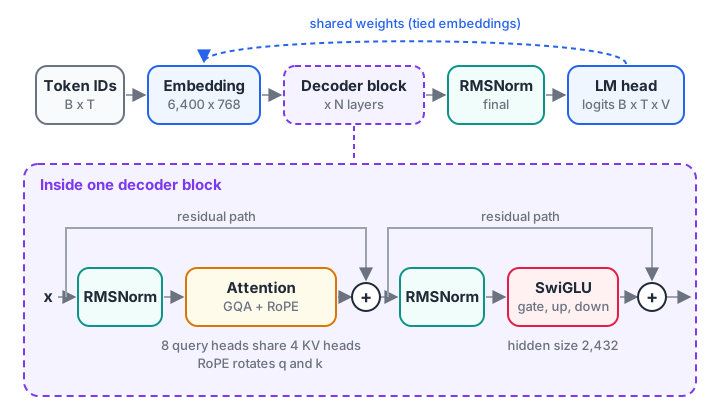
The block in the dashed box is repeated N times. The output head reuses the embedding matrix, which saves millions of parameters.

How many parameters will your model have?

Count before you code. Almost all parameters sit in four places: the embedding table, the attention projections, the feed-forward layers, and (if untied) the output head.

Python

def count_params(vocab, d, layers, heads, kv_heads, ffn, tied=True):
    hd = d // heads
    attn = d * heads * hd + 2 * d * kv_heads * hd + heads * hd * d   # q, k, v, o
    mlp = 3 * d * ffn                                               # gate, up, down
    norms = 2 * d                                                   # two RMSNorms
    per_layer = attn + mlp + norms
    emb = vocab * d
    total = emb + layers * per_layer + d + (0 if tied else emb)
    return total, emb, layers * attn, layers * mlp

for name, cfg in {"small variant": (6400, 512, 8, 8, 4, 1408),
                  "running example": (6400, 768, 8, 8, 4, 2432)}.items():
    total, emb, attn, mlp = count_params(*cfg)
    print(f"{name:15s} total {total/1e6:5.1f}M | embedding {emb/1e6:4.1f}M "
          f"| attention {attn/1e6:4.1f}M | feed-forward {mlp/1e6:4.1f}M")

The feed-forward layers hold most of the weights. That is normal: attention decides where to look, while the feed-forward layers store much of what the model knows.

Should a small model be deep or wide?

At a fixed parameter budget, research on sub-billion models such as MobileLLM found that deeper, narrower models tend to beat shallow, wide ones. Don't go too narrow, though.

Below a hidden size of about 512, each head gets very few dimensions to work with. For a first build, 8 to 16 layers at hidden size 512 to 768 is a safe range.

How does RMSNorm work?

RMSNorm rescales each token's vector so its root-mean-square is 1, then multiplies by a learned gain. Unlike LayerNorm, it doesn't subtract the mean or add a bias, so it is cheaper and, in practice, works as well. It comes from Zhang and Sennrich, 2019.

Python

import numpy as np

def rms_norm(x, weight, eps=1e-5):
    rms = np.sqrt(np.mean(x ** 2, axis=-1, keepdims=True) + eps)
    return x / rms * weight

x = np.array([[2.0, -4.0, 6.0, 0.5],
              [0.01, 0.02, -0.01, 0.03]])          # one large token, one tiny token
w = np.ones(4)
y = rms_norm(x, w)
print(np.round(y, 3))
print("RMS after norm:", np.round(np.sqrt((y ** 2).mean(axis=-1)), 3))

Both tokens come out at about the same scale, whatever size they went in. The tiny token lands just under 1 because eps, which prevents division by zero, matters when values are this small. Placing the norm before each sub-layer ("pre-norm") keeps gradients stable in deep stacks, which is why every modern LLM does it.

How does RoPE encode positions?

Rotary position embedding (RoPE), from Su and colleagues, 2021, doesn't add a position vector. It rotates each pair of dimensions of the query and key by an angle proportional to the token's position, with a different speed for each pair.

When you take the dot product of a rotated query and key, the angles subtract, so the attention score depends only on their distance, not on where they sit in the sentence.

Python

import numpy as np

def rope(x, base=10000.0):
    seq, dim = x.shape
    half = dim // 2
    inv_freq = base ** (-np.arange(half) / half)          # one speed per pair
    ang = np.arange(seq)[:, None] * inv_freq[None, :]     # (seq, dim/2)
    cos, sin = np.cos(ang), np.sin(ang)
    x1, x2 = x[:, :half], x[:, half:]                     # "rotate half" layout
    return np.concatenate([x1 * cos - x2 * sin, x2 * cos + x1 * sin], axis=-1)

rng = np.random.default_rng(0)
q_vec, k_vec = rng.normal(size=8), rng.normal(size=8)
Q = rope(np.tile(q_vec, (12, 1)))      # same query content at every position
K = rope(np.tile(k_vec, (12, 1)))
for qp, kp in [(3, 1), (7, 5), (11, 9), (7, 1)]:
    print(f"query at {qp:2d}, key at {kp:2d}, distance {qp-kp}: score {Q[qp] @ K[kp]:+.4f}")
print("length kept:", round(np.linalg.norm(q_vec), 4), round(np.linalg.norm(Q[5]), 4))

Distance 2 gives the same score at positions 3, 7 and 11. Rotation also keeps the vector's length, so RoPE never distorts the content.

Can RoPE handle longer text than it was trained on?

Not by default. A model trained on 1,024-token blocks has never seen the larger angles that appear beyond that, and quality drops sharply. Methods such as YaRN rescale the rotation frequencies at inference time so a model can stretch to several times its training length.

Many small models also set a large rope_base, such as 1,000,000 instead of 10,000, so angles grow more slowly. You will test length extrapolation in evaluating a small LLM.

Quick check

Why does RoPE make attention depend on relative position?

What is grouped-query attention?

In standard multi-head attention, each of the 8 query heads has its own key head and value head. Grouped-query attention (Ainslie and colleagues, 2023) lets several query heads share one key/value head. With 8 query heads and 4 KV heads, as in the running example, each pair of query heads reads the same keys and values.

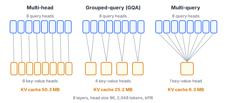
GQA sits between the two extremes: almost the quality of full multi-head attention, with a fraction of its KV cache.

The saving matters at inference, when the model stores every past key and value in the KV cache:

Python

import numpy as np

B, T, d, heads, kv_heads = 1, 6, 768, 8, 4
hd = d // heads
k = np.random.default_rng(1).normal(size=(B, kv_heads, T, hd))
k_expanded = np.repeat(k, heads // kv_heads, axis=1)       # each KV head serves 2 query heads
print("stored K:", k.shape, "-> used by attention:", k_expanded.shape)

layers, ctx, bytes_per = 8, 2048, 2                         # bf16
for name, kvh in [("multi-head", 8), ("grouped (GQA)", 4), ("multi-query", 1)]:
    cache = 2 * layers * ctx * kvh * hd * bytes_per          # K and V
    print(f"{name:14s} KV cache for 2,048 tokens: {cache/1e6:5.1f} MB")

The model stores only 4 KV heads and repeats them when it computes attention, so the cache is half the size of full multi-head attention. Going down to 2 KV heads would halve it again, at a small cost in quality.

Quick check

With 12 query heads and 4 KV heads, how many query heads share each KV head?

What is SwiGLU?

The feed-forward layer of the original transformer was Linear → ReLU → Linear. SwiGLU, from Shazeer, 2020, uses three matrices: a gate passed through the SiLU (swish) function, an up projection, their element-wise product, then a down projection. The gate learns which features to let through for each token.

Python

import numpy as np

def silu(x):
    return x / (1 + np.exp(-x))

rng = np.random.default_rng(2)
d, ffn = 8, 24                      # real models: about 8/3 * d, rounded to a multiple of 64
W_gate, W_up = rng.normal(size=(d, ffn)) * 0.3, rng.normal(size=(d, ffn)) * 0.3
W_down = rng.normal(size=(ffn, d)) * 0.3
x = rng.normal(size=(3, d))         # 3 tokens
h = silu(x @ W_gate) * (x @ W_up)   # gated hidden layer
y = h @ W_down
print("in", x.shape, "hidden", h.shape, "out", y.shape)
print("fraction of hidden units nearly shut by the gate:", round(float(np.mean(np.abs(silu(x @ W_gate)) < 0.05)), 2))

Because SwiGLU has three matrices instead of two, its hidden size is usually about 8/3 of the model width rather than 4 times, which keeps the parameter count the same.

For width 768 that gives exactly 2,048. The running example goes a little wider, to 2,432 (about 3.2 times the width, and a multiple of 64), spending about 7M extra parameters on feed-forward capacity.

The full model in PyTorch

Here is a complete, minimal decoder-only model with all four pieces. It targets PyTorch 2.x and uses scaled_dot_product_attention, which picks a fast fused kernel on recent GPUs.

Python

import torch
import torch.nn as nn
import torch.nn.functional as F
from dataclasses import dataclass

@dataclass
class Config:
    vocab_size: int = 6400
    dim: int = 768
    n_layers: int = 8
    n_heads: int = 8
    n_kv_heads: int = 4
    ffn_dim: int = 2432
    max_seq_len: int = 1024
    rope_base: float = 10000.0
    norm_eps: float = 1e-5

class RMSNorm(nn.Module):
    def __init__(self, dim, eps):
        super().__init__()
        self.eps, self.weight = eps, nn.Parameter(torch.ones(dim))
    def forward(self, x):
        xf = x.float()
        xf = xf * torch.rsqrt(xf.pow(2).mean(-1, keepdim=True) + self.eps)
        return xf.type_as(x) * self.weight

def rope_tables(head_dim, max_len, base):
    inv = 1.0 / base ** (torch.arange(0, head_dim, 2).float() / head_dim)
    ang = torch.outer(torch.arange(max_len).float(), inv)
    ang = torch.cat([ang, ang], dim=-1)                  # (max_len, head_dim)
    return ang.cos(), ang.sin()

def apply_rope(x, cos, sin):                             # x: (B, H, T, hd)
    T = x.shape[-2]
    x1, x2 = x.chunk(2, dim=-1)
    rotated = torch.cat([-x2, x1], dim=-1)
    return (x * cos[:T] + rotated * sin[:T]).type_as(x)

class Attention(nn.Module):
    def __init__(self, c):
        super().__init__()
        self.h, self.kv, self.hd = c.n_heads, c.n_kv_heads, c.dim // c.n_heads
        self.q = nn.Linear(c.dim, self.h * self.hd, bias=False)
        self.k = nn.Linear(c.dim, self.kv * self.hd, bias=False)
        self.v = nn.Linear(c.dim, self.kv * self.hd, bias=False)
        self.o = nn.Linear(self.h * self.hd, c.dim, bias=False)
    def forward(self, x, cos, sin):
        B, T, _ = x.shape
        q = self.q(x).view(B, T, self.h, self.hd).transpose(1, 2)
        k = self.k(x).view(B, T, self.kv, self.hd).transpose(1, 2)
        v = self.v(x).view(B, T, self.kv, self.hd).transpose(1, 2)
        q, k = apply_rope(q, cos, sin), apply_rope(k, cos, sin)
        k = k.repeat_interleave(self.h // self.kv, dim=1)   # GQA: share KV heads
        v = v.repeat_interleave(self.h // self.kv, dim=1)
        y = F.scaled_dot_product_attention(q, k, v, is_causal=True)
        return self.o(y.transpose(1, 2).reshape(B, T, -1))

class SwiGLU(nn.Module):
    def __init__(self, c):
        super().__init__()
        self.gate = nn.Linear(c.dim, c.ffn_dim, bias=False)
        self.up = nn.Linear(c.dim, c.ffn_dim, bias=False)
        self.down = nn.Linear(c.ffn_dim, c.dim, bias=False)
    def forward(self, x):
        return self.down(F.silu(self.gate(x)) * self.up(x))

class Block(nn.Module):
    def __init__(self, c):
        super().__init__()
        self.norm1, self.attn = RMSNorm(c.dim, c.norm_eps), Attention(c)
        self.norm2, self.mlp = RMSNorm(c.dim, c.norm_eps), SwiGLU(c)
    def forward(self, x, cos, sin):
        x = x + self.attn(self.norm1(x), cos, sin)
        return x + self.mlp(self.norm2(x))

class TinyLM(nn.Module):
    def __init__(self, c):
        super().__init__()
        self.cfg = c
        self.embed = nn.Embedding(c.vocab_size, c.dim)
        self.layers = nn.ModuleList([Block(c) for _ in range(c.n_layers)])
        self.norm = RMSNorm(c.dim, c.norm_eps)
        self.lm_head = nn.Linear(c.dim, c.vocab_size, bias=False)
        self.lm_head.weight = self.embed.weight              # weight tying
        cos, sin = rope_tables(c.dim // c.n_heads, c.max_seq_len, c.rope_base)
        self.register_buffer("cos", cos, persistent=False)
        self.register_buffer("sin", sin, persistent=False)
        self.apply(self._init)

    def _init(self, m):
        if isinstance(m, (nn.Linear, nn.Embedding)):
            nn.init.normal_(m.weight, mean=0.0, std=0.02)

    def forward(self, idx, targets=None):
        x = self.embed(idx)
        for layer in self.layers:
            x = layer(x, self.cos, self.sin)
        logits = self.lm_head(self.norm(x))
        loss = None
        if targets is not None:
            loss = F.cross_entropy(logits.float().reshape(-1, logits.size(-1)),
                                   targets.reshape(-1), ignore_index=-100)
        return logits, loss

if __name__ == "__main__":
    cfg = Config()
    model = TinyLM(cfg)
    print(f"{sum(p.numel() for p in model.parameters())/1e6:.1f}M parameters")
    x = torch.randint(0, cfg.vocab_size, (2, 64))
    logits, loss = model(x[:, :-1], x[:, 1:])
    print(logits.shape, round(loss.item(), 2))   # loss starts near ln(6400) = 8.76

Run it on CPU first. It should print about 63.9M parameters, a logits shape of (2, 63, 6400) and a loss near 8.8, which is what a model guessing uniformly over 6,400 tokens scores. A starting loss far above that usually means a bad initialisation.

Adding a mixture-of-experts layer

To try a mixture-of-experts model, replace SwiGLU in some blocks with a small router plus, say, 4 SwiGLU experts, and send each token to its top 1 or 2 experts.

Total parameters grow but active parameters per token stay similar. Expect training to be noticeably slower in plain PyTorch, because tokens must be sorted by expert; add an auxiliary load-balancing loss so one expert doesn't take every token.

Common architecture mistakes

Forgetting the causal mask. Without is_causal=True the model sees the answer, the loss drops to almost zero, and generation is garbage.
Mixing RoPE layouts. "Rotate half" and "interleaved pairs" are both valid, but export tools expect one. Use rotate half if you plan to convert to Hugging Face or GGUF format in the deployment tutorial.
Heads that don't divide. n_heads must be divisible by n_kv_heads, and dim by n_heads.
Untied embeddings on a tiny model. Untying adds another 4.9M parameters to the 64M model for little gain.

Key takeaways

A small LLM is embeddings, N identical pre-norm decoder blocks, a final RMSNorm and a tied output head.
RMSNorm rescales without centring; RoPE rotates queries and keys so scores depend on distance.
GQA shares KV heads across query heads, cutting the KV cache several times.
SwiGLU uses three matrices with a hidden size about 8/3 of the width.
Next, train this model in pretraining an LLM from scratch. If you'd rather build it alongside classmates, look at Generative AI training at Debugshala, Old Palasia.

FAQ

What architecture do small LLMs use today?

Most small open models use a decoder-only transformer with pre-norm RMSNorm, rotary position embeddings, grouped-query attention and a SwiGLU feed-forward layer, often with tied input and output embeddings. Some add mixture-of-experts layers. The 2017 design with LayerNorm, learned positions and ReLU is now rare.

How do I calculate the number of parameters in a transformer?

Add the embedding table (vocab × width), and for each layer the attention projections (query, key, value and output) plus the feed-forward matrices (three of width × hidden for SwiGLU). Norms add very little. The calculator above does this and matches PyTorch's own count.

Why use RMSNorm instead of LayerNorm?

RMSNorm skips the mean subtraction and bias, so it is simpler and slightly faster, and in practice it trains as well as LayerNorm. Placing it before each sub-layer (pre-norm) keeps training stable in deep stacks.

Is grouped-query attention worse than multi-head attention?

Slightly, in some studies, but the gap is small, and GQA cuts the KV cache by the ratio of query heads to KV heads. That makes long-context inference much cheaper, so most recent models use it.

Where can I learn Generative AI in a classroom in Indore?

Debugshala, an IT training institute in Old Palasia, Indore, offers a Generative AI course in English and Hindi with a free demo class. It accepts fresh graduates and non-IT learners. You can also check your understanding with free quizzes on Debugshala Test.

Small LLM Architecture in Code: RMSNorm, RoPE, GQA and SwiGLU

What does a small LLM architecture look like?

How many parameters will your model have?

Should a small model be deep or wide?

How does RMSNorm work?

How does RoPE encode positions?

Can RoPE handle longer text than it was trained on?

What is grouped-query attention?

What is SwiGLU?

The full model in PyTorch

Adding a mixture-of-experts layer

Common architecture mistakes

Key takeaways

FAQ

What architecture do small LLMs use today?

How do I calculate the number of parameters in a transformer?

Why use RMSNorm instead of LayerNorm?

Is grouped-query attention worse than multi-head attention?

Where can I learn Generative AI in a classroom in Indore?

Go further with the Generative AI Course at Debugshala

Keep learning

Build a Small LLM from Scratch: The Complete 2026 Roadmap

Train a BPE Tokenizer for Your LLM: Vocab Size and Chat Tokens

LLM Training Data Preparation: Pretraining and Chat Datasets