

DPO Training Tutorial: Align a Small LLM with Preference Pairs
Train a small LLM with DPO: preference pair format, the loss from log-probs, choosing beta, a PyTorch loop and the reward curves that warn of trouble.
Think of a music teacher in Indore listening to a student sing the same line twice. She doesn't perform the perfect version herself. She just says, "The second take was better than the first." Over many such comparisons, the student's singing shifts towards what she likes.
That is much easier for the teacher than writing a perfect example every time. Judging is cheaper than creating.
Direct Preference Optimization uses exactly this shortcut to tune a language model.
What is DPO training?
DPO (Direct Preference Optimization) is a fine-tuning method that trains an LLM directly on preference pairs, increasing the probability of the preferred answer relative to the rejected one while a frozen reference model keeps it close to where it started.
Mapping the analogy: the two takes are the chosen and rejected answers. The student's singing before lessons is the reference model, a frozen copy of your SFT checkpoint. The student who keeps practising is the policy model you train. How firmly the teacher corrects is beta.
DPO was introduced by Rafailov et al. (2023). It reaches the same goal as classic RLHF, but replaces the reward model and PPO loop with a single classification-style loss. For where it fits among post-training methods, see SFT vs RLHF vs GRPO.
In this series, DPO comes after supervised fine-tuning and optional knowledge distillation. Your model can already chat. DPO nudges which of its possible answers it prefers.
How does the DPO loss work?
For each pair, you need four numbers: the log-probability of the chosen answer and of the rejected answer, under both the policy and the reference.
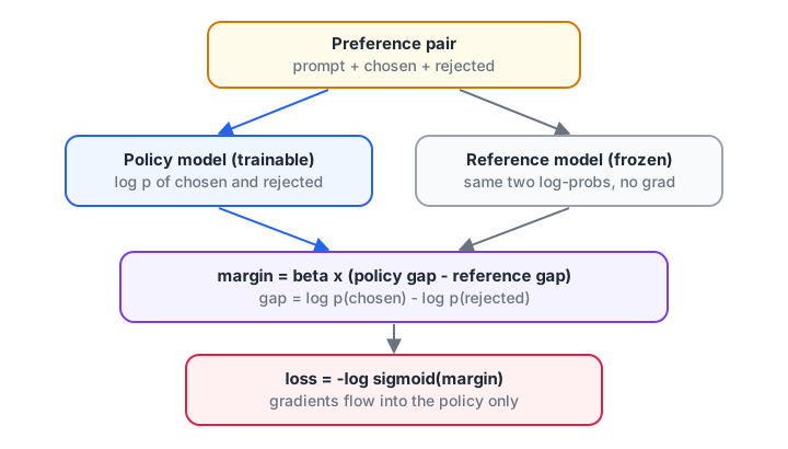
Only the policy receives gradients. The reference is run with gradients off, or its log-probs are computed once and cached.
The "gap" is how much more a model likes the chosen answer than the rejected one. DPO rewards the policy for widening its gap beyond the reference's gap. Written out:
policy_gap    = log p_policy(chosen) - log p_policy(rejected)
reference_gap = log p_ref(chosen)    - log p_ref(rejected)
loss          = -log sigmoid( beta * (policy_gap - reference_gap) )
Because everything is measured relative to the reference, a pair the SFT model already handled well gives little gradient. Pairs where the policy still prefers the wrong answer give the most.
The preference data format
Each line in your jsonl file holds the prompt once, plus a good and a bad assistant reply. This is the prompt, chosen, rejected layout planned in data preparation, written as chat messages:
{"prompt":   [{"role": "user", "content": "Explain RAM in one line."}],
 "chosen":   [{"role": "assistant", "content": "RAM is the fast, temporary memory a computer uses for the programs it is running right now."}],
 "rejected": [{"role": "assistant", "content": "RAM RAM is memory memory that is a computer thing used in computers."}]}
Where do pairs come from? You have three practical options:
| Source | How it works | Fit for a small model |
|---|---|---|
| Public preference datasets | Download pairs labelled by people or strong models | Easy start, but answers may be far above your model's level |
| LLM-as-a-judge | A strong model picks the better of two answers | Scales well; see LLM-as-a-judge |
| On-policy pairs | Sample two answers from your own SFT model, then rank them | Usually the best fit, because both answers are within reach |
On-policy pairs matter for tiny models. If the chosen answer is a polished essay your 64M model could never write, its log-probability is so low that the pair teaches very little.
Render prompt plus chosen, and prompt plus rejected, with the same chat template you used in SFT. Mask the prompt tokens so only the assistant reply counts, exactly like the SFT loss mask.
Compute DPO step by step in Python
Step 1: score one answer
A sequence log-probability is the sum of the answer tokens' log-probs. The prompt tokens are masked out.
import numpy as np

# Per-token log-probs for one tokenised chat: 5 prompt tokens, then 4 answer tokens
token_logps = np.array([-2.1, -0.4, -3.0, -1.2, -0.8,   -0.9, -0.3, -1.6, -0.2])
loss_mask   = np.array([0,    0,    0,    0,    0,      1,    1,    1,    1])

seq_logp = (token_logps * loss_mask).sum()
print("answer tokens:", int(loss_mask.sum()))
print(f"log p(answer | prompt) = {seq_logp:.2f}")
print(f"probability of the whole answer = {np.exp(seq_logp):.4f}")
print(f"mean log-prob per answer token = {seq_logp / loss_mask.sum():.2f}")
Summing, not averaging, is the standard DPO choice. It does mean longer answers have more negative totals, which is one source of length bias.
Step 2: the loss and implicit rewards
The quantity beta * (log p_policy - log p_ref) is called the implicit reward. Logging it for chosen and rejected answers is the best way to see what DPO is doing.
import numpy as np

def dpo_loss(pol_c, pol_r, ref_c, ref_r, beta=0.1):
    # Implicit rewards: how much the policy moved away from the reference
    r_c = beta * (pol_c - ref_c)
    r_r = beta * (pol_r - ref_r)
    margin = r_c - r_r
    loss = np.log1p(np.exp(-margin))     # equals -log(sigmoid(margin))
    return loss.mean(), r_c.mean(), r_r.mean(), (margin > 0).mean()

# Sequence log-probs (sum over answer tokens) for 4 preference pairs
ref_c = np.array([-42.0, -30.5, -55.1, -18.2])
ref_r = np.array([-40.3, -29.0, -50.7, -20.1])

steps = {
    "start (policy = reference)": (ref_c, ref_r),
    "after some training":        (ref_c + 3.0, ref_r - 4.0),
    "over-trained":               (ref_c - 6.0, ref_r - 30.0),
}
for name, (pc, pr) in steps.items():
    loss, rc, rr, acc = dpo_loss(pc, pr, ref_c, ref_r)
    print(f"{name:<28} loss={loss:.3f} chosen_r={rc:+.2f} rejected_r={rr:+.2f} acc={acc:.2f}")
At the start the loss is ln 2, about 0.693, because policy and reference are identical. After some training, chosen rewards rise and rejected rewards fall.
Look at the last row: the loss is lowest, but the chosen reward has gone negative. The model learned to dislike rejected answers by lowering the probability of everything. That is a warning sign, not a success.
Step 3: choose beta
Beta sets how quickly a pair stops contributing. The gradient weight for a pair is sigmoid(-beta * gap), so a large beta saturates fast.
import numpy as np

# Same log-ratio gap, different beta: how strongly does DPO still push?
gap = np.array([0.0, 5.0, 10.0, 20.0, 40.0])   # (pol_c - ref_c) - (pol_r - ref_r)

print("gap   " + "  ".join(f"beta={b:<4}" for b in (0.05, 0.1, 0.5)))
for g in gap:
    row = []
    for beta in (0.05, 0.1, 0.5):
        # gradient weight = sigmoid(-beta * gap): near 1 = still learning, near 0 = done
        w = 1 / (1 + np.exp(beta * g))
        row.append(f"{w:9.3f}")
    print(f"{g:4.0f} " + "  ".join(row))
With beta=0.5, a pair stops teaching once the gap reaches about 10 nats. With beta=0.1, the model keeps being pushed further. Values from 0.1 to 0.5 are common; 0.1 is a sensible default.
Quick check
At the very start of DPO training, when the policy equals the reference, what is the loss?
The margin is 0, so the loss is -log sigmoid(0) = ln 2, about 0.693.
A minimal DPO training loop in PyTorch
This loop starts from the TinyLM SFT checkpoint. Each batch holds chosen and rejected sequences stacked together, the first half chosen and the second half rejected, with a 0/1 mask that marks the answer tokens (aligned with ids, not shifted).
import copy
import torch
import torch.nn.functional as F
from model import Config, TinyLM

ckpt = torch.load("checkpoints/sft_epoch1.pt", map_location="cuda")    # your final SFT checkpoint
cfg = Config(**ckpt["config"])
policy = TinyLM(cfg).cuda()
policy.load_state_dict(ckpt["model"])
policy.train()
reference = copy.deepcopy(policy).eval().requires_grad_(False)          # frozen copy
opt = torch.optim.AdamW(policy.parameters(), lr=5e-7, weight_decay=0.0)
beta = 0.1

def seq_logps(model, ids, mask):
    logits, _ = model(ids)                             # TinyLM returns (logits, loss)
    logits = logits.float()[:, :-1]
    logps = torch.gather(F.log_softmax(logits, -1), 2, ids[:, 1:, None]).squeeze(-1)
    return (logps * mask[:, 1:]).sum(-1)               # sum over answer tokens only

for step, (ids, mask) in enumerate(loader):            # ids: [2B, L]
    ids, mask = ids.cuda(), mask.cuda()
    with torch.autocast("cuda", dtype=torch.bfloat16):
        pol = seq_logps(policy, ids, mask)
        with torch.no_grad():
            ref = seq_logps(reference, ids, mask)
    B = ids.size(0) // 2
    pol_c, pol_r, ref_c, ref_r = pol[:B], pol[B:], ref[:B], ref[B:]
    margin = beta * ((pol_c - ref_c) - (pol_r - ref_r))
    loss = -F.logsigmoid(margin).mean()

    opt.zero_grad(set_to_none=True)
    loss.backward()
    torch.nn.utils.clip_grad_norm_(policy.parameters(), 1.0)
    opt.step()
    if step % 50 == 0:
        print(step, f"loss={loss.item():.3f}",
              f"chosen_r={(beta * (pol_c - ref_c)).mean().item():+.3f}",
              f"rejected_r={(beta * (pol_r - ref_r)).mean().item():+.3f}",
              f"acc={(margin > 0).float().mean().item():.2f}")

torch.save({"model": policy.state_dict(), "config": cfg.__dict__}, "checkpoints/dpo_last.pt")
Settings that work as a starting point for a model this size:
- Learning rate: far below SFT, around 1e-7 to 1e-6 for full fine-tuning. Small models forget their SFT skills quickly at higher rates.
- Epochs: one pass is usually enough. More epochs over a few thousand pairs overfit fast.
- Sequence length: the same as SFT, often 512 to 1,024 tokens.
- Memory: two copies of the model and four forward passes per pair, so expect about twice the memory of SFT at the same batch size.
A 64M model with a few thousand pairs finishes in minutes to under an hour on one consumer GPU. Treat that as a rough estimate; your sequence length and batch size change it a lot.
If your model is already in Hugging Face Transformers format (the export is covered in the last article of this series), the DPOTrainer in the TRL library runs the same algorithm with logging built in.
What to watch while DPO trains
The loss alone is misleading. Plot three curves: mean chosen reward, mean rejected reward and their margin.
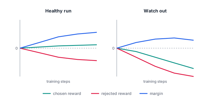
Both rewards falling means the model is lowering the probability of every answer, which often makes generations worse.
Then read real outputs. Generate answers to the same 20 prompts before and after DPO. If answers grow longer, more repetitive or start to break the chat format, lower the learning rate or stop earlier. The small LLM evaluation guide shows how to set up that comparison.
Quick check
The DPO loss keeps falling, but both chosen and rejected rewards are going down. What does that suggest?
A healthy run keeps the chosen reward roughly flat or rising while the rejected reward falls.
Common DPO mistakes
- Skipping SFT. DPO refines a model that can already answer. On a base model, both answers have tiny probabilities and nothing useful happens.
- Reference not frozen. If the reference updates too, the gaps cancel and training silently does nothing.
- Learning rate copied from SFT. This is the most common reason a small model starts to babble after DPO.
- Length-biased pairs. If chosen answers are always longer, the model simply learns "longer is better".
- Different templates for chosen and rejected. Any formatting difference becomes an easy shortcut the model learns instead of quality.
Once DPO is stable, you can try online methods that let the model explore, covered in PPO and GRPO for LLMs. If you prefer learning in a classroom, the Generative AI programme Debugshala runs in English and Hindi is one option.
Key takeaways
- DPO trains on chosen and rejected pairs using a frozen reference model and a single loss.
- Implicit rewards,
beta * (log p_policy - log p_ref), are the numbers to plot. - Use on-policy pairs, a learning rate far below SFT and about one epoch.
- On a small model, DPO shapes style and safety more than correctness.
FAQ
Is DPO better than RLHF with PPO?
DPO is simpler and cheaper, because it needs no reward model and no sampling loop, so it is usually the first choice for small teams. PPO-style RLHF can explore new answers online and may reach better results on large models, but it is harder to tune and needs more memory.
How many preference pairs do I need for DPO?
A few thousand good pairs is a reasonable start for a small model; public preference datasets are often tens of thousands of pairs. Quality and relevance matter more than size. Pairs where both answers come from your own model usually teach more than pairs with answers far above its level.
Why is my DPO model getting worse?
The usual causes are a learning rate that is too high, too many epochs, or pairs with a length or format bias. Check whether the chosen reward is falling along with the rejected reward. If it is, lower the learning rate, train for fewer steps, or clean the pairs.
What does beta do in DPO?
Beta controls how strongly the policy may move away from the reference model. A higher beta makes each pair saturate faster and keeps the model closer to its SFT behaviour. A lower beta allows larger changes. Most runs use a value between 0.1 and 0.5.
Is there a generative AI course in Indore with a free demo?
Debugshala's Generative AI course runs at its Old Palasia campus in Indore, with teaching in English and Hindi and a free demo class first. Courses accept fresh graduates and non-IT learners. You can try practice questions on Debugshala Test before you join.
From the team behind this site
Go further with the Generative AI Course at Debugshala
These tutorials are written by Debugshala, a training and placement institute at Old Palasia, Indore. The classroom course adds live mentoring, real projects and interview preparation.
- Offline classes at Old Palasia, Indore
- Free demo class before you pay
- Non-IT, fresher and year-gap friendly
- Placement assistance
700+ students placed · 200+ hiring partners · 4.9★ Google rating
