Pretrain an LLM from Scratch: Loss, LR Schedule and Checkpoints

Pretrain a small LLM in PyTorch: next-token loss, warmup and cosine LR, bf16, gradient accumulation, checkpoints, resuming and reading the loss curve.

A child in Indore hears thousands of hours of Hindi and English before anyone teaches grammar. Nobody explains rules. She just keeps guessing the next word in conversations, notices when she's wrong, and adjusts. Years later she speaks fluently, though she still can't do your income-tax return.

Pretraining is that childhood. The thousands of hours are billions of tokens of text. Each guess is a next-token prediction, noticing the mistake is the loss, and adjusting is a gradient step. Fluency comes from pretraining; skills like following instructions come later in supervised fine-tuning.

What is LLM pretraining?

LLM pretraining is the first and largest training stage, in which a language model with random weights learns to predict the next token across a large text corpus, producing a base model that can continue any text but does not yet follow instructions.

This is stage 5 of the build-an-LLM roadmap. You need the token files from data preparation and the TinyLM model from small LLM architecture. For where pretraining sits among all training stages, see how LLMs are trained.

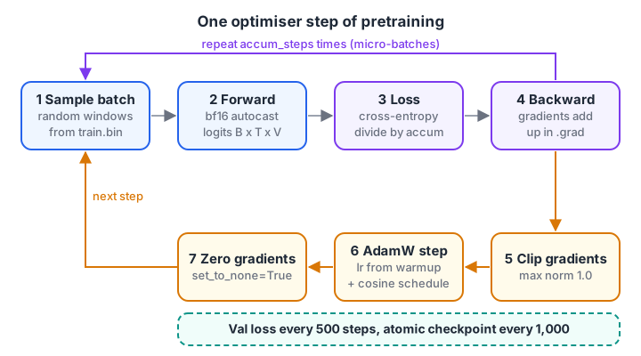
LLM pretraining loop: sample a batch of token windows, forward pass with bf16 autocast, next-token cross-entropy loss, backward pass accumulated over micro-batches, gradient clipping, AdamW step with a scheduled learning rate, and periodic evaluation and checkpoints

One optimiser step runs several forward and backward passes. Evaluation and checkpoints happen every few hundred steps.

How is the pretraining loss calculated?

At every position, the model outputs a score (logit) for each of the 6,400 tokens in the vocabulary. Softmax turns the scores into probabilities, and the loss is the negative log of the probability given to the token that actually came next. Average that over every position in the batch and you have cross-entropy loss.

Python

import numpy as np

def cross_entropy(logits, target):
    z = logits - logits.max()                      # numerical stability
    log_probs = z - np.log(np.exp(z).sum())
    return -log_probs[target]

vocab = 6400
print(f"random model, uniform guess: loss = {cross_entropy(np.zeros(vocab), 42):.3f}"
      f"  (ln {vocab} = {np.log(vocab):.3f})")

for p in [0.01, 0.1, 0.5, 0.9]:
    logits = np.full(vocab, 0.0)
    logits[42] = np.log(p * (vocab - 1) / (1 - p))   # make P(token 42) = p
    loss = cross_entropy(logits, 42)
    print(f"P(correct)={p:4.2f} -> loss {loss:.3f}, perplexity {np.exp(loss):7.1f}")

That first line is your sanity check: a fresh model should start near 8.8. Perplexity is exp(loss), roughly "how many tokens the model is choosing between". A loss of 3.0 means a perplexity of about 20. The evaluation tutorial uses it to compare checkpoints.

Quick check

A freshly initialised model with a 6,400-token vocabulary should start pretraining with a loss of about what?

Which hyperparameters should you use?

These are reasonable starting values for the 64M running example in this series (and its 27M variant). They are common choices in published small-model recipes, not tuned optima, so treat them as a first run.

Setting	Starting value	Why
Optimiser	AdamW, betas (0.9, 0.95)	Standard for transformers; 0.95 reacts faster to loss spikes
Peak learning rate	6e-4 (try 3e-4 to 1e-3)	Small models tolerate higher LR than large ones
Warmup	1 to 3 percent of steps	Avoids huge early updates while Adam's statistics settle
Decay	Cosine to 10 percent of peak	Smooth slowdown that fine-tunes the final weights
Weight decay	0.1 on matrices, 0 on norms	Regularises without shrinking norm gains
Gradient clipping	1.0	Caps rare huge gradients from odd batches
Sequence length	512 to 1,024 tokens	Enough context for short documents
Tokens per step	64k to 256k	Micro-batch × sequence length × accumulation × GPUs
Precision	bf16 autocast	Halves activation memory without loss scaling

What does a warmup and cosine schedule look like?

Python

import math

peak, floor, warmup, total = 6e-4, 6e-5, 400, 20000

def lr_at(step):
    if step < warmup:
        return peak * (step + 1) / warmup
    progress = (step - warmup) / (total - warmup)
    return floor + 0.5 * (peak - floor) * (1 + math.cos(math.pi * progress))

for s in [0, 200, 399, 2000, 5000, 10000, 15000, 19999]:
    bar = "#" * int(lr_at(s) / peak * 40)
    print(f"step {s:5d}  lr {lr_at(s):.2e}  {bar}")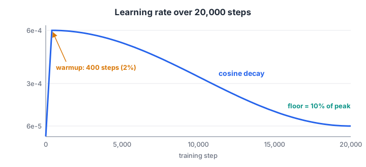

Warmup and cosine learning rate schedule for LLM pretraining: the learning rate rises linearly for 400 steps to 6e-4, then follows a cosine curve down to 6e-5 at step 20,000

The warmup is short. Most of the run is spent on the long cosine descent.

How many steps and how long will it take?

Work out tokens per step first, then divide your token budget by it.

Python

micro_batch, seq_len, accum, gpus = 32, 512, 4, 1
tokens_per_step = micro_batch * seq_len * accum * gpus
budget = 1.28e9                         # 20 tokens/param for the 64M model
steps = budget / tokens_per_step
for tok_per_sec in [60_000, 120_000, 200_000]:     # measure yours from the log
    hours = budget / tok_per_sec / 3600
    print(f"{tokens_per_step:,} tokens/step, {steps:,.0f} steps, "
          f"at {tok_per_sec:,} tok/s -> {hours:4.1f} h")

The script below rounds this to 20,000 steps, about 1.31B tokens. The tokens-per-second figures are placeholders. Run 100 steps, read the real number from your log, and redo the sum. Throughput depends on the GPU, sequence length, whether fused attention kernels are used, and whether torch.compile is on.

Quick check

Micro-batch 16, sequence length 1,024, accumulation 8, one GPU. How many tokens per optimiser step?

Why use gradient accumulation?

A micro-batch of 32 sequences of 512 tokens may be all your GPU's memory can hold. Gradient accumulation runs several micro-batches, adds up their gradients, and only then takes one optimiser step. Mathematically, it gives the same gradient as one big batch, provided you divide each micro-batch loss by the number of accumulation steps.

Python

import numpy as np

rng = np.random.default_rng(0)
X, y = rng.normal(size=(8, 3)), rng.normal(size=8)
w = np.zeros(3)

def grad(Xb, yb, w):                      # gradient of mean squared error
    return 2 * Xb.T @ (Xb @ w - yb) / len(yb)

full = grad(X, y, w)
accum = sum(grad(X[i:i+2], y[i:i+2], w) / 4 for i in range(0, 8, 2))   # 4 micro-batches
print("one batch of 8   :", np.round(full, 5))
print("4 x micro-batch 2:", np.round(accum, 5))
print("equal:", np.allclose(full, accum))

Forgetting the division makes the effective learning rate four times too high, a common cause of early divergence.

The pretraining script in PyTorch

This script trains TinyLM from model.py. It samples random windows from the uint16 token file, uses bf16 autocast, accumulates gradients, clips them, follows the warmup-plus-cosine schedule, evaluates on held-out tokens, and writes an atomic checkpoint it can resume from.

Python

import math, os, time
import numpy as np
import torch
from model import Config, TinyLM

train_bin, val_bin = "data/pretrain_train.bin", "data/pretrain_val.bin"
seq_len, micro_batch, accum_steps = 512, 32, 4      # 65,536 tokens per step
max_steps, warmup_steps = 20000, 400
peak_lr, min_lr, weight_decay, grad_clip = 6e-4, 6e-5, 0.1, 1.0
eval_every, save_every, out_dir = 500, 1000, "checkpoints"
device = "cuda" if torch.cuda.is_available() else "cpu"
dtype = torch.bfloat16                                # float16 + GradScaler on older GPUs
torch.manual_seed(42)

def get_batch(path):
    data = np.memmap(path, dtype=np.uint16, mode="r")
    ix = torch.randint(len(data) - seq_len - 1, (micro_batch,))
    x = torch.stack([torch.from_numpy(data[i:i + seq_len].astype(np.int64)) for i in ix])
    y = torch.stack([torch.from_numpy(data[i + 1:i + 1 + seq_len].astype(np.int64)) for i in ix])
    return x.to(device, non_blocking=True), y.to(device, non_blocking=True)

cfg = Config(max_seq_len=seq_len)
model = TinyLM(cfg).to(device)
decay = [p for p in model.parameters() if p.dim() >= 2]      # matrices, embeddings
no_decay = [p for p in model.parameters() if p.dim() < 2]    # norm weights
optimizer = torch.optim.AdamW(
    [{"params": decay, "weight_decay": weight_decay},
     {"params": no_decay, "weight_decay": 0.0}],
    lr=peak_lr, betas=(0.9, 0.95), eps=1e-8)

def lr_at(step):
    if step < warmup_steps:
        return peak_lr * (step + 1) / warmup_steps
    progress = (step - warmup_steps) / max(1, max_steps - warmup_steps)
    return min_lr + 0.5 * (peak_lr - min_lr) * (1 + math.cos(math.pi * min(progress, 1.0)))

os.makedirs(out_dir, exist_ok=True)
ckpt_path, start_step = os.path.join(out_dir, "pretrain_last.pt"), 0
if os.path.exists(ckpt_path):                              # resume after a crash
    ckpt = torch.load(ckpt_path, map_location=device)
    model.load_state_dict(ckpt["model"])
    optimizer.load_state_dict(ckpt["optimizer"])
    start_step = ckpt["step"] + 1
    print("resumed from step", ckpt["step"])

@torch.no_grad()
def eval_loss(batches=20):
    model.eval()
    losses = []
    for _ in range(batches):
        x, y = get_batch(val_bin)
        with torch.autocast(device_type=device, dtype=dtype):
            _, loss = model(x, y)
        losses.append(loss.item())
    model.train()
    return sum(losses) / len(losses)

model.train()
t0 = time.time()
for step in range(start_step, max_steps):
    for group in optimizer.param_groups:
        group["lr"] = lr_at(step)

    for _ in range(accum_steps):
        x, y = get_batch(train_bin)
        with torch.autocast(device_type=device, dtype=dtype):
            _, loss = model(x, y)
        (loss / accum_steps).backward()           # gradients add up across micro-batches

    norm = torch.nn.utils.clip_grad_norm_(model.parameters(), grad_clip)
    optimizer.step()
    optimizer.zero_grad(set_to_none=True)

    if step % 50 == 0:
        dt, t0 = time.time() - t0, time.time()
        tok_s = 50 * accum_steps * micro_batch * seq_len / dt if step > start_step else 0
        print(f"step {step:5d} | loss {loss.item():.3f} | lr {lr_at(step):.2e} "
              f"| grad norm {norm:.2f} | {tok_s:,.0f} tok/s")
    if step % eval_every == 0 or step == max_steps - 1:
        print(f"step {step:5d} | val loss {eval_loss():.3f}")
    if step % save_every == 0 or step == max_steps - 1:
        torch.save({"model": model.state_dict(), "optimizer": optimizer.state_dict(),
                    "step": step, "config": cfg.__dict__}, ckpt_path + ".tmp")
        os.replace(ckpt_path + ".tmp", ckpt_path)   # never leave a half-written file

Three details are easy to miss. The checkpoint stores the optimiser state, without which a resumed run starts with an empty Adam memory and the loss jumps. The .tmp then os.replace pattern means a crash during saving never corrupts your last good checkpoint. And the val loss uses tokens the model never trains on.

To speed things up on a recent GPU, wrap the model with model = torch.compile(model) after moving it to the device; see the PyTorch compile docs.

Training on more than one GPU

For two or more GPUs, use PyTorch's DistributedDataParallel (DDP): each GPU runs the same script on different batches and gradients are averaged automatically. Launch it with torchrun:

Terminal

torchrun --standalone --nproc_per_node=2 pretrain.py

Inside the script you call torch.distributed.init_process_group("nccl"), wrap the model in DistributedDataParallel, give each rank a different random seed for get_batch, and save checkpoints only from rank 0. The DDP tutorial covers the details. Remember that tokens per step doubles, so you may halve accum_steps.

How to read the pretraining loss curve

A healthy run falls from about 8.8 to below 5 within the first few hundred steps, as the model learns common words and spacing. Then the curve bends and falls slowly for the rest of the run.

Train and val loss should stay close. Final values depend heavily on your data and tokenizer, so compare runs with each other, not with numbers from other projects.

Sample text every evaluation, too. Early on you'll see random tokens, then real words, then grammatical sentences on the right topic, with facts that are often wrong.

Symptom	Likely cause	Fix
Loss stays near 8.8	Learning rate far too low, or labels not shifted	Check `y` is `x` shifted by one; raise LR
Loss becomes NaN	fp16 overflow or LR too high	Use bf16, lower LR, keep clipping on
Sudden spikes, then recovery	A bad batch or LR slightly too high	Lower peak LR by a third; inspect data near the spike
Train falls, val rises	Too few unique tokens, repeated epochs	Add data or stop earlier
Loss near 0 within minutes	Causal mask missing, model sees the future	Set `is_causal=True`
Out of memory	Micro-batch or sequence too large	Halve micro-batch, double `accum_steps`

Before any long run, overfit a single batch for 200 steps. The loss should drop close to zero. If it can't, the bug is in your code, not your data.

If you'd rather learn with trainers in person, consider a classroom Generative AI programme that accepts year-gap learners in Indore.

Key takeaways

Pretraining minimises next-token cross-entropy; a fresh model starts near ln(vocab size).
Use AdamW, a short warmup, cosine decay to 10 percent, bf16, clipping at 1.0 and weight decay on matrices only.
Gradient accumulation reaches a large effective batch on a small GPU; divide the loss by the accumulation steps.
Save model and optimiser state atomically so you can resume.
The base model continues text but doesn't chat yet. Next comes supervised fine-tuning, or first check it with evaluation.

FAQ

What learning rate should I use to pretrain a small LLM?

Start with a peak of about 6e-4 for a 25M to 100M model, with a warmup over 1 to 3 percent of steps and cosine decay to a tenth of the peak. If the loss spikes repeatedly, lower it by a third; if it falls very slowly and smoothly, try up to 1e-3.

How long does pretraining a small LLM take on one GPU?

Divide your token budget by your measured tokens per second. A 27M model on about 0.5B tokens typically needs one to a few hours on a modern consumer GPU, while the 64M running example on 1.3B tokens needs roughly two to ten hours, depending on throughput. Measure throughput in the first 100 steps to get your real figure.

What is a good loss value for LLM pretraining?

There is no universal target, because loss depends on the tokenizer and the data. A fresh model starts near ln(vocab size). What matters is a smooth fall, train and val loss staying close, and lower val loss than your previous run on the same data and tokenizer.

Should I use bf16 or fp16 for LLM training?

Use bf16 if your GPU supports it (NVIDIA Ampere, the RTX 30 series, and newer). It has the same range as fp32, so it rarely overflows and needs no gradient scaler. On older GPUs, use fp16 with torch.amp.GradScaler, and watch for NaN losses.

Where can I practise deep learning concepts like this?

Free practice quizzes on Debugshala Test cover coding and aptitude topics. If you prefer learning in person, Debugshala, a training institute in Old Palasia, Indore, runs a Generative AI course in English and Hindi with a free demo class first.

Pretrain an LLM from Scratch: Loss, LR Schedule and Checkpoints

What is LLM pretraining?

How is the pretraining loss calculated?

Which hyperparameters should you use?

What does a warmup and cosine schedule look like?

How many steps and how long will it take?

Why use gradient accumulation?

The pretraining script in PyTorch

Training on more than one GPU

How to read the pretraining loss curve

Key takeaways

FAQ

What learning rate should I use to pretrain a small LLM?

How long does pretraining a small LLM take on one GPU?

What is a good loss value for LLM pretraining?

Should I use bf16 or fp16 for LLM training?

Where can I practise deep learning concepts like this?

Go further with the Generative AI Course at Debugshala

Keep learning

Supervised Fine-Tuning Tutorial: From Base LLM to Chat Model

LLM Knowledge Distillation: Teacher Data and Reasoning Traces

DPO Training Tutorial: Align a Small LLM with Preference Pairs