

LLM Decoding Strategies: Greedy, Beam Search and Sampling
Compare LLM decoding strategies: greedy decoding, beam search, sampling, constrained and speculative decoding, with runnable Python toy examples.
Imagine you are driving from Vijay Nagar to Rajwada in the evening. At every junction you can see only the next stretch of road. One strategy: always take whichever road looks emptiest right now. It feels smart, but an empty road can lead into a jam two turns later.
A cleverer driver keeps two or three possible routes in mind, follows each a little further, and drops the ones that start to look bad. A third driver, out for fun, sometimes picks a less obvious turn just to see a different part of the city.
An LLM faces a junction at every token. How it chooses the road is its decoding strategy.
What is a decoding strategy in an LLM?
Mapping the drive: each junction is one generation step. The road options are the next-token probabilities. Taking the emptiest road is greedy decoding. Tracking a few routes is beam search. Picking turns with some randomness is sampling. The whole trip is the output sequence, and what you really want is the best whole trip, not the best first turn.
A decoding strategy is the rule an LLM uses to choose tokens from its predicted probability distributions, step by step, to build the output text, with the goal of producing a sequence that is likely, useful or varied enough for the task.
The model, explained in what is an LLM, only produces probabilities. Decoding is a separate piece of code wrapped around it, so the same model can behave very differently depending on the strategy. The knobs inside sampling, such as temperature and top-p, were covered in LLM generation parameters; this article compares the strategies themselves.
Greedy decoding: always take the top token
Greedy decoding picks the single most likely token at every step. It is fast, simple and fully deterministic. It also has a blind spot: a slightly less likely first token can lead to a far more likely sentence.
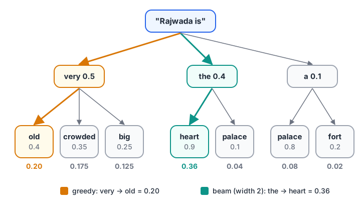
Greedy decoding grabs the best first word and ends with a worse sentence; beam search keeps a second option alive and finds the better one.
The probability of a whole sequence is the product of its step probabilities. This toy model completes "Rajwada is" in two words:
LM = {
    "":             {"very": 0.5, "the": 0.4, "a": 0.1},
    "very":         {"old": 0.4, "crowded": 0.35, "big": 0.25},
    "the":          {"heart": 0.9, "palace": 0.1},
    "a":            {"palace": 0.8, "fort": 0.2},
}   # toy model: next-word probabilities after "Rajwada is ..."

def greedy(steps=2):
    words, prob = [], 1.0
    for _ in range(steps):
        options = LM[" ".join(words)]
        best = max(options, key=options.get)       # always take the top word
        prob *= options[best]
        words.append(best)
    return words, prob

def all_paths(prefix=(), prob=1.0, steps=2):
    if steps == 0:
        yield list(prefix), prob; return
    for w, p in LM[" ".join(prefix)].items():
        yield from all_paths(prefix + (w,), prob * p, steps - 1)

words, p = greedy()
print("greedy :", "Rajwada is", " ".join(words), f"  P={p:.2f}")
best_words, best_p = max(all_paths(), key=lambda x: x[1])
print("best   :", "Rajwada is", " ".join(best_words), f"  P={best_p:.2f}")
Greedy picks "very" because 0.5 beats 0.4, but every word after "very" is uncertain. "the" was a weaker start that leads to "heart" with 0.9 confidence. The full search found it, but checking every path is impossible for a real model: with a 100,000-token vocabulary, even a 3-token output has 10^15 paths.
Greedy decoding also tends to repeat itself in long outputs ("The poha is good. The poha is good."), because a likely phrase keeps reinforcing itself.
Quick check
Why can greedy decoding miss the most likely sentence?
A weaker first token can lead to much more confident later tokens; greedy never explores that path.
Quick check
Beam search with a beam width of 1 is the same as which strategy?
Keeping only one candidate at each step means always taking the single best token.
Beam search: keep several candidates alive
Beam search is the practical middle ground. At each step it keeps the beam width (say 2 to 5) best partial sentences, extends each one by every possible next token, scores the results, and again keeps only the best few.
- Start with an empty sentence.
- Extend every kept sentence with each possible next token.
- Score each new sentence by the sum of its log-probabilities.
- Keep the top width sentences and drop the rest.
- Repeat until all kept sentences end or hit the length limit, then return the best.
Log-probabilities are used because multiplying many small numbers underflows; adding logs is the same thing, safely.
import math

LM = {
    "":             {"very": 0.5, "the": 0.4, "a": 0.1},
    "very":         {"old": 0.4, "crowded": 0.35, "big": 0.25},
    "the":          {"heart": 0.9, "palace": 0.1},
    "a":            {"palace": 0.8, "fort": 0.2},
}

def beam_search(width, steps=2):
    beams = [([], 0.0)]                            # (words, sum of log-probabilities)
    for step in range(steps):
        candidates = []
        for words, score in beams:
            for w, p in LM[" ".join(words)].items():
                candidates.append((words + [w], score + math.log(p)))
        beams = sorted(candidates, key=lambda b: b[1], reverse=True)[:width]
        kept = " | ".join(f"{' '.join(w)} ({math.exp(s):.2f})" for w, s in beams)
        print(f"  step {step + 1}, keep {width}: {kept}")
    return beams[0]

for width in [1, 2]:
    print(f"beam width {width}:")
    words, score = beam_search(width)
    print(f"  -> Rajwada is {' '.join(words)}  P={math.exp(score):.2f}\n")
With width 1, beam search is identical to greedy. With width 2, "the" survives step 1 and wins at step 2.
Length normalisation and where beam search fits
Every extra token multiplies in another number below 1, so raw beam scores favour short outputs. Implementations divide the score by the length raised to a power, often called the length penalty, to level the field.
Beam search shines when there is roughly one right answer: machine translation, speech-to-text, summarising into a fixed format. For open-ended chat it often produces bland, generic and repetitive text, because the most probable sentence is usually the dullest.
Sampling: controlled randomness
Sampling draws each token at random according to its probability. A 0.4-probability token is chosen about 40% of the time. Temperature, top-p and min-p shape and trim the distribution before the draw.
import numpy as np

LM = {
    "":     {"very": 0.5, "the": 0.4, "a": 0.1},
    "very": {"old": 0.4, "crowded": 0.35, "big": 0.25},
    "the":  {"heart": 0.9, "palace": 0.1},
    "a":    {"palace": 0.8, "fort": 0.2},
}

def sample(rng, temperature=1.0):
    words = []
    for _ in range(2):
        options = LM[" ".join(words)]
        p = np.array(list(options.values())) ** (1 / temperature)   # same as logits / T
        words.append(rng.choice(list(options), p=p / p.sum()))
    return " ".join(words)

rng = np.random.default_rng(3)
for t in [0.5, 1.0]:
    outs = [sample(rng, t) for _ in range(300)]
    top = sorted(set(outs), key=outs.count, reverse=True)
    print(f"T={t}: {len(top)} different endings; most common:",
          ", ".join(f"'{o}' x{outs.count(o)}" for o in top[:3]))
Even at temperature 0.5 there are several endings, and the most likely sentence appears only about 4 times in 10. This is why asking a chat assistant the same question twice can give two different, equally fine answers.
Sampling also enables self-consistency: generate several answers and take the most common final result, which is covered in prompting techniques for reasoning.
Constrained and speculative decoding
Two more techniques sit on top of any base strategy: one controls what may be generated, the other how fast.
Constrained decoding: forcing a valid format
Sometimes the output must follow strict rules: valid JSON, one of five labels, an integer. Constrained decoding masks out every token that would break the rule before choosing, so invalid output becomes impossible rather than merely unlikely.
import numpy as np

# the model's top candidates for the next token after '{"age": '
vocab = ['"twenty', '20', 'about', '2', 'unknown', '21', 'null']
probs = np.array([0.34, 0.22, 0.15, 0.12, 0.08, 0.06, 0.03])

def allowed(token):
    return token.isdigit()          # a JSON schema says "age" must be an integer

mask = np.array([allowed(t) for t in vocab])
constrained = np.where(mask, probs, 0)
constrained /= constrained.sum()

print("unconstrained pick:", vocab[int(np.argmax(probs))])
print("allowed tokens    :", [t for t, m in zip(vocab, mask) if m])
print("constrained pick  :", vocab[int(np.argmax(constrained))],
      f"(renormalised prob {constrained.max():.2f})")
Real systems compile a JSON schema or grammar into a state machine that allows only tokens keeping the output valid.
This is how "structured output" and "JSON mode" features work under the hood; the practical side is in structured output and JSON prompting. Constraints can only choose among what the model offers, so a confused model will produce valid but wrong output.
Speculative decoding: same output, faster
Every strategy above calls the big model once per token, and that is slow. Speculative decoding uses a small, fast draft model to guess several tokens ahead, then runs the big model once to check all of them in parallel.
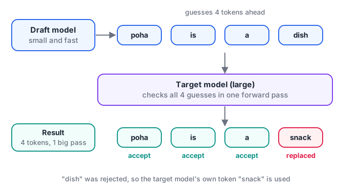
The draft model guesses cheaply; the target model checks the guesses in one pass and keeps the ones it agrees with.
Accepted tokens are kept, and the first rejected one is replaced with the big model's own choice. With the standard acceptance rule, the output follows the big model's distribution exactly, so quality is unchanged; only speed improves, often by around 2 to 3 times when the draft guesses well. It is one of several methods in LLM inference optimisation.
Decoding strategies compared
| Strategy | Deterministic? | Diversity | Speed | Best for |
|---|---|---|---|---|
| Greedy | Yes | None | Fastest | Short factual answers, extraction, code completion |
| Beam search | Yes | Low | Slower (width × work) | Translation, transcription, fixed formats |
| Sampling (temperature, top-p) | No (unless seeded) | Adjustable | Fast | Chat, creative writing, brainstorming |
| Constrained decoding | Follows base strategy | Limited by rules | Small overhead | JSON, labels, schema-bound output |
| Speculative decoding | Matches base strategy | Matches base strategy | Faster | Any of the above when latency matters |
Decoding strategies in Hugging Face transformers
In transformers, the arguments to generate() select the strategy. This needs the library and a downloaded model, so it runs on your machine, not in the browser. Pass do_sample=False explicitly, because many models ship a generation config that turns sampling on by default.
# greedy decoding
out = model.generate(**inputs, max_new_tokens=60, do_sample=False)

# beam search: 4 beams, avoid repeating any 3-gram
out = model.generate(**inputs, max_new_tokens=60, do_sample=False,
                     num_beams=4, length_penalty=1.0, no_repeat_ngram_size=3,
                     early_stopping=True)

# sampling
out = model.generate(**inputs, max_new_tokens=60, do_sample=True,
                     temperature=0.7, top_p=0.9)

# speculative (assisted) decoding with a small draft model sharing the tokenizer
out = model.generate(**inputs, max_new_tokens=60, assistant_model=draft_model)
print(tokenizer.decode(out[0], skip_special_tokens=True))
Common mistakes with decoding strategies
- Using beam search for chat. It makes answers flat and repetitive. Sample instead.
- Assuming greedy is "most accurate". It is most probable per step, not necessarily best overall, and it loops on long outputs.
- Huge beam widths. Quality often gets worse past about 5 to 10 beams, while cost keeps rising.
- Trusting constraints for correctness. A schema guarantees shape, not truth. Validate values too.
Key takeaways
- Decoding turns probabilities into text; the same model behaves differently under different strategies.
- Greedy is fast and deterministic but short-sighted and prone to loops.
- Beam search keeps several candidates and suits tasks with one right answer; it is a poor fit for chat.
- Sampling gives natural, varied text and is the default for assistants.
- Constrained decoding enforces formats, and speculative decoding speeds up generation without changing the output distribution.
Next in the series, how to run LLMs locally puts these strategies to work on your own machine. If you want to drill the concepts, solve more GenAI MCQs on Debugshala Test.
FAQ
What decoding strategy does ChatGPT use?
Exact settings of commercial chat products are not fully published, but chat assistants generally use sampling with temperature and top-p filtering. That is why the same question can produce different wordings. APIs let you lower the temperature for more consistent answers.
Is beam search better than greedy decoding?
For tasks with one correct output, such as translation, beam search usually finds higher-probability and better sequences than greedy. For open-ended writing it often produces bland, repetitive text. It also costs more compute, roughly in proportion to the beam width.
What is the difference between decoding and sampling?
Decoding is the general process of turning a model's probabilities into tokens. Sampling is one decoding strategy, the one that picks tokens at random according to their probabilities. Greedy decoding and beam search are other decoding strategies that involve no randomness.
Does speculative decoding reduce output quality?
No, not with the standard verification rule. The large model checks every drafted token and replaces the first one it disagrees with, so the final text follows the large model's own distribution. The only change is speed, which depends on how often the draft model guesses correctly.
Where can I learn LLM decoding and inference in Indore?
Debugshala teaches LLM internals, decoding and inference optimisation in its classroom Generative AI programme at Old Palasia, in English and Hindi, with placement assistance. A free demo is available first; see an instructor-led Generative AI course in Indore.
From the team behind this site
Go further with the Generative AI Course at Debugshala
These tutorials are written by Debugshala, a training and placement institute at Old Palasia, Indore. The classroom course adds live mentoring, real projects and interview preparation.
- Offline classes at Old Palasia, Indore
- Free demo class before you pay
- Non-IT, fresher and year-gap friendly
- Placement assistance
700+ students placed · 200+ hiring partners · 4.9★ Google rating
